Nick Haubrich

Follymarket: How to judge Polymarket's forecasting ability?

Introduction

A recurring topic through the US’s 2024 presidential election was the prominence and accuracy of online betting markets. As the largest, Polymarket received the most news attention despite its illegality in the US¹. With 60-40 odds in favor of Trump as the polls closed, Polymarket outperformed polling-based models from Nate Silver (50-50), FiveThirtyEight (50-49), and The Economist (56-43). Somehow, international bettors, including a millionaire French whale and some unscrupulous US citizens with VPNs, beat the experts and left with money to show for it.

So just how smart is Polymarket? A single event hardly justifies a whole model. To properly assess the betting platform, we need more data. Polymarket presumably has a log of every transaction buried on-chain, but thankfully they also host a REST API with plenty of information. Just a dash of Python and a heap of patience is all that’s needed to scrape the price info for closed markets. I obtained data from ??? markets over the range December 27, 2023 to December 30, 2024, which is most of the easily-accessible data². Each market contains the share price at 10-minute intervals up to a month prior to closing . These are all binary markets, so as a convention I always use the price of the side that resolves true.

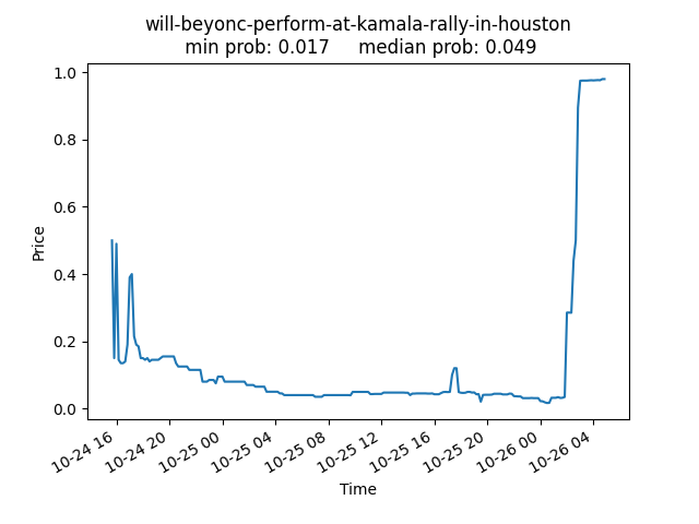
For example, here’s the pricing of whether or not Beyonce would appear and perform at Kamala Harris’s Houston rally. In this cherry-picked case, the market leaned towards the wrong result up until Queen Bey walked on stage. (Traders may have over-corrected from Beyonce’s previous no-show at the DNC.)

As share prices are bound between 0 and 1, it’s natural to interpret them as the probability the market assigns to the outcome. This seemingly basic point has attracted a surprising amount of academic discussion, e.g. this paper which concludes that prediction markets don’t exactly represent an averaging of beliefs, but the discrepancy is usually small. We’ll ignore these subtleties, and instead see if prices empirically behave like probabilities.

Accuracy

The simplest way to judge a prediction is by its accuracy, i.e. putting a high price on the outcome that happens. The inherent difficulty is that it’s based off observed outcomes, not the true underlying probability. A 100% confident prediction that comes true is highly accurate, even if the event is a long shot that happens to pan out once. Having repeated outcomes (i.e. multiple coinflips) of the same event strengthens the case for accuracy as the one-metric-to-rule-them-all, but this is the opposite situation of Polymarket’s many varied bets.

The Brier score, forecasters’ term for mean squared error (MSE), is one way to quantify accuracy. For \(N\) binary prediction probabilities (or prices) \(p\) and outcomes \(y\), the Brier score is

Simply computing this over the price data gives a score of .074, which is the same value a single 73% prediction would get. Off the bat, Polymarket beats coinflips and magic 8 balls.

However, some markets are longer than others and therefore contain more predictions. Arguably, the score above over-emphasizes the slower markets, which may not change significantly in each 10-minute sampling interval, and de-emphasize faster markets. In some sense, this is an issue with the fixed-rate sampling, and it would be nicer to have a fixed number of points for each market regardless of its duration. Lacking that, the next best thing is to apply a weighting inversely proportional to each market’s length, i.e. a weighted Brier Score,

for \(M\) markets of varying length \(N_j\). This Weighted Brier Score is 0.13 (matching a single \(p\)=64% value), a higher (worse) value than before, demonstrating the impact of the weighting. I’d argue that the weighted version leads to better statements, e.g. the accuracy of markets halfway before closing rather than 1 day before closing. FiveThirtyEight’s self-evaluation uses a similar methodology.

We can also plot the average price over the market’s duration. The mean is shown alongside bands covering 68% and 95% of the distribution. (As a reminder, our convention always uses the price of the outcome that happened.) This plot alone shows how the markets become more accurate over time. After an initial lurch as the market finds an equilibrium, prices gradually increase until a rapid ascent as the outcome is all but confirmed. Note the mean price hovers around the 64% probability from the Weighted Brier Score. The spread around the mean is large, as indicated by the \(\pm1\sigma\) and \(\pm2\sigma\) quantiles. The average accuracy says little about any particular prediction.

Calibration

Calibration, which quantifies how closely the predicted odds act like probabilities in aggregate, gives another perspective. Many political election sites tout their well-calibrated models (see Election Betting Odds’ or FiveThirtyEight’s where a candidate given a 1-in-4 chance will actually win about 25% of the time. While calibration is important for interpreting and making decisions off the model, achieving a high calibration isn’t as impressive as it may seem. For instance, one can achieve perfect calibration by assigning every binary outcome a 50% chance. The accuracy will be terrible, but exactly half of the outcomes assigned even odds will come true.

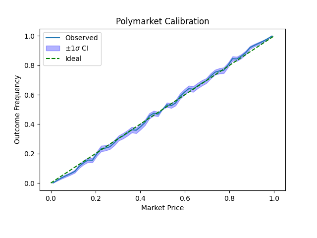
To compute the calibration of our Polymarket data, we take the distribution of prices and compare the frequencies of each price at \(p\) and \(1-p\). We can approximate these frequencies \(f_p\) by histogramming the price data (weighted by inverse market length, like before) into small bins. The market is perfectly calibrated if \(\frac{f_p}{f_{p}+f_{1-p}}=p\) at all price points, i.e. the assigned probability occurs at the rate it is assigned.

In the calibration plot shown, values below the ideal line correspond to overconfident predictions. But by-and-large the prices are well-calibrated. Even the tails, which are rife with market inefficiencies (transaction costs, delays resolving outcomes, etc.), only slightly deviate from the ideal. The \(\pm1\sigma\) confidence intervals are constructed by a 500-partition bootstrap resampling³.

There’s a hidden connection between the Brier score and calibration. The Brier score can be decomposed into two terms. The first is a calibration score, which is minimized when predicted probabilities match their outcome frequencies. The second term is the refinement, which accounts for how scattered the predictions. (A larger spread gives a lower score, i.e. the perfectly-calibrated coinflip model would incur a large penalty.) Mathematically, this is stated as

for forecast probabilities \(p\), binary outcomes \(y\), and outcome frequencies \(f\). While the Brier score sums over all \(N\) predictions, the other two sums are over the prediction probabilities in \(K\) bins, in the same way the calibration plot was made, with \(n_k\) accounting for the number of predictions in each bin.

One way to view this calibration metric is as the MSE of the calibration curve to the ideal dotted line in the plot above. The refinement is slightly more complex to understand. If we assume a perfectly-calibrated forecast, then \(f_k\) is restricted to be a diagonal line, and \(f_k(1-f_k)\) is a downward-facing parabola peaking at \(j=0.5\). The highest (worst) score would be if all predictions fell at the maximum, and the score is reduced by predictions closer to either extreme. The refinement, then, rewards extreme predictions that preserve the calibration.

After applying the now-standard inverse-length reweighting⁴, our dataset yields a calibration term of .0005, against a refinement of .13. Thus, the vast majority of the Brier score comes from calibrated forecasts that miss the mark.

Direct Comparison

A particularly Bayesian (or as Nate Silver might say, riverian) metric for predictions is to gauge its profitability ⁵, assuming one can bet on the forecast as stated odds. For predictions such as Polymarket, this is merely coming full circle. Given an alternate forecast and some basic trading strategy, one can quantify the profit or deficit over any range of markets and timespan.

Defensive forecasting pokes a hole in this view (though no worse a hole than the pitfalls with accuracy and calibration). Like the 50-50 calibration example, there’s a simple strategy guaranteed to never lose money: agree with your opponent. That is, given the distribution of how much your opponent would wager at any forecasted probability, pick your forecast so they wager $0. If no such point exists, your opponent is willing to wager money on one side no matter the odds, so forecast that outcome with probability 1. This amounts to copying their forecast.

The original paper on Defensive Forecasting uses it to connect game theory to statistics, showing that countering certain strategies correspond to statistical measures. While this is a formally interesting result, it only works exactly against a single fully-specified strategy, which is a far cry from practice. The broad point is that any fixed strategy can be trivially gamed, highlighting the need for multiple statistical metrics when assessing predictions.

One example by Harry Crane (from his own 2018 comparison of FiveThirtyEight and PredictIt) achieves calibration only by over-correcting for past effects, with no insight to the future. Crane then evaluates the two markets on a head-to-head betting scheme. By placing pretend wagers on one market using the probabilities of the other, the markets can be compared for identical events. Since wagers can be placed on different events at the same time, the amount placed on each event is determined by a multi-bet Kelly Criterion. The markets can then be compared based on relative portfolio performance.

This approach is both intuitive and robust. Synchronizing the two markets surely takes some work, but otherwise it’s fairly straightforward. The main issue that plagues it is that the Kelly criterion assumes independent probabilities, but Polymarket (and other markets) have bets ranging from moderately correlated (e.g. state election turnout) to extremely correlated (e.g. presidential election winner vs who will be inaugurated).

Conclusion

The fundamental difficulty with evaluating predictions is that, almost by definition, their true probability is unknown. Most statistical tools rely on a notion of similarity to group occurrences by commonality, and from these groups the underlying probability can be estimated. Many experiments and observations are well-suited to this kind of analysis. One-off prediction markets are not. They cover unique one-off events that are almost unthinkable to replicate. Their inner workings, being an aggregation of individual’s opinions, is a black box rivaling that of large language models.

In such a case, one must fall back on simpler metrics. Anyone touting calibration alone, being so easy to achieve, should not be taken seriously. The Brier score, a standard for a reason, combines accuracy and calibration into a single number. The main benefit is to allow easy comparisons across models and datasets. At the very least, a model can be compared against random chance. Polymarket undoubtedly is better than pure noise. Relative comparisons, such as betting-based metrics, open the door to more extensive comparisons but require a second model and more intensive data-wrangling.

The point of any metric is to simplify. Since any metric will throw out information, none can be considered perfect. Instead, metrics need to be chosen to answer the question at hand. Brier score and calibration plots answer basic questions, but complicated models can go wrong in ways that require deeper investigation. For a first analysis, the simplest will have to do.

Lest anyone is in danger of having too much faith in Polymarket’s ability after this analysis, below are some of the largest misses of the past year.

<180 MPs vote to impeach Yoon?

NHL Rangers vs. Predators 2024-12-17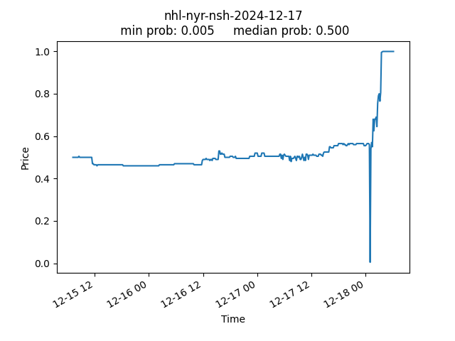

Will there be a US Government shutdown before 2025?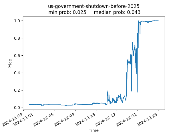

Will Gukesh Dommaraju win Game 14 of the World Chess Championship?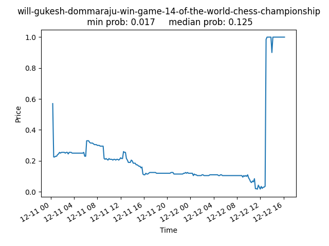

Will Harris win New Mexico by 6+ points?

Will Kamala Harris go on SNL?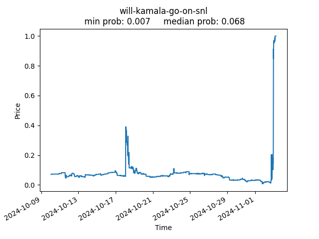

Will Matt Eberflus be the next head coach fired?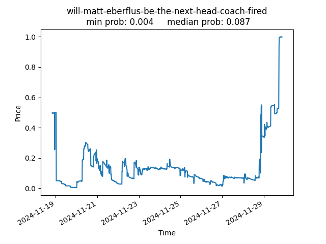

Code for this project can be found at github.com/nhaubrich/Follymarket.